Most Machine Learning projects usually go like this:
- Get a dataset.
- Create a model trying to predict something.
- Modify the model until you get good metrics.
- Profit.
Luckily for you, this project is unique compared to most data science projects.
I am proud of this project because it shows how I:
- Worked with a large and imperfect data set.
- Created a model that performed great at the task of predicting XG (expected goals).
- Deployed the model to a website that creates visualizations of XG (expected goals).
- Received feedback from new HaxBall players on my model.
Goal: Create and deploy machine learning models to predict “expected goals” (XG) in the online game HaxBall.
I'll explain a couple of things before I get into the technical details of what I worked on.
What is HaxBall
HaxBall is an online physics-based multi-player soccer game.
Below is a short animation of the game being played.
GIF credit to GIFHY.
Each player is a circle that can kick and interact with the ball. You can move using WASD (or arrows) and space to kick the ball.
What is XG (Expected Goals)?
Below is a short video explaining what expected goals means in the context of soccer.
Summary of the video:
XG is the probability of a given kick resulting in a goal and can be used to create higher-order metrics, for both offense and defense.
XG helps describe the match, but does not attempt to solve soccer or predict the results. For example, if a team has a high cumulative XG score through the match but doesn’t score any goals, this would mean the team was applying pressure through the match and had chances to score but did not score.
XG does not account for who is taking the shot, one definition of elite strikers are those who score more than their XG suggests.
Some criticisms of XG in soccer include undermining the value of clinical strikers. In other terms, strikers who can stay calm under pressure in positions close to the goal but don’t outperform their XG consistently. We know there is no such thing as a 100% chance of a goal.
Predicting XG in HaxBall
Predicting XG using Machine Learning was a multi-step process.
The steps below outline the type of work I performed:
- Exploratory data analysis
- Feature Engineering
- Comparison of Models and Features
- Discussion and Results
Usually, this would not be something anyone could do in one sitting. (Maybe at a hackathon with 3 red bulls.)
Exploratory data analysis
Before creating a Machine Learning model, I had to do some exploratory data analysis to understand the types of data we had collected. This was the beginning of brainstorming for the feature engineering I would do later. The main goal of this data analysis was to see what types of data we had and how the data was obtained.
We had collected data on hundreds of goals, thousands of different matches and millions of player positions.
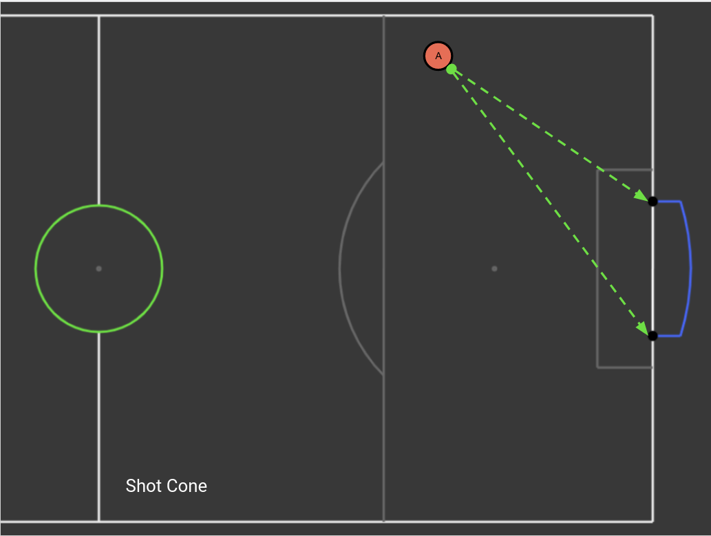
Here are two example schemas that I used often.
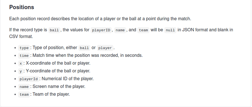
The complete data schema for the data I worked with is on the HaxClass repository. This repository also contains the source code for Headless API that recorded data from matches.
Once I had a good understanding of the data collected I started creating different features, the inputs to the model. I had to brainstorm features that would make the model better at predicting XG. This process of brainstorming, generating and evaluating features, was a process I repeated a couple of times before I picked my final set of features.
Feature Engineering
Feature engineering is when you use domain knowledge to extract features from raw data using data mining techniques. The purpose of a feature is to make the problem easier to understand in the context of the problem. - Feature Engineering Wikipedia
I had to draw comparisons between soccer and HaxBall to create features that would make the model better at predicting XG. Haxball is less complex than soccer, this made the task of predicting XG a bit easier. In Haxball, players can only kick and block the ball, while in soccer players can make different types of headers and trick shots, etc.
Some ideas for features I wanted to use as input:
- Goal Distance (numerical): the distance from the ball to the goal.
- Goal Angle (numerical): the angle in radians between the line of the shot and the goal line, 0 for parallel to the goal line, pi/2 for perpendicular to the goal line.
- Defender within a distance (numerical): The number of defenders within a predefined distance from the ball.
- Closest Defender (numerical): The distance to the closest defender.
- Players within a box (numerical): The number of players in a rectangle coming out from the goal to the ball.
- Player in box (boolean): Whether there are any players within the rectangle created by defenders_within_box.
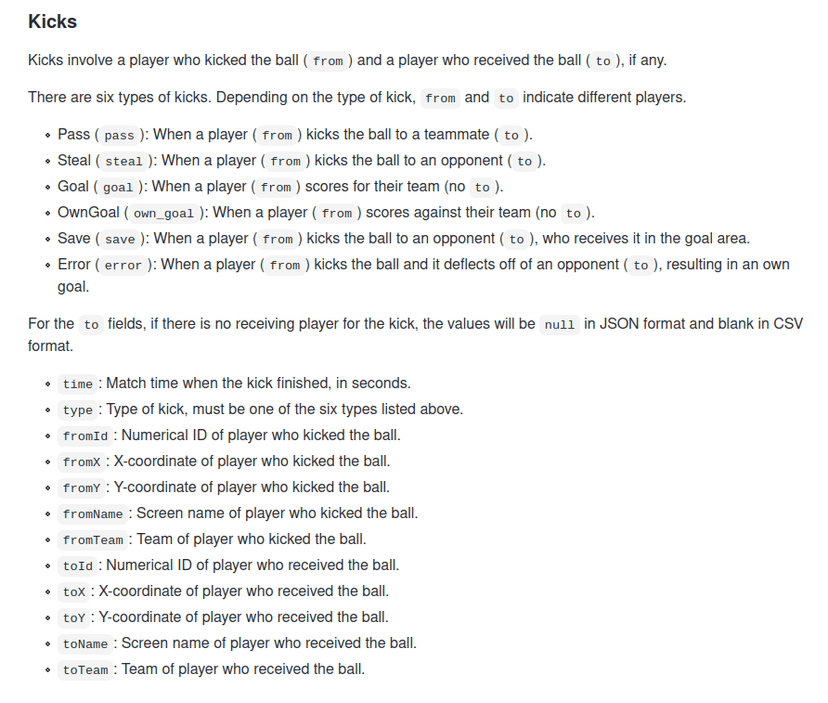
- Players within the shot (numerical): The number of players in a cone from the goalposts to the ball.
- Player in shot (boolean): Whether there are any players within the rectangle created by defenders_within_shot.
- Ball speed (numerical): Speed of the ball within a 1 second interval using distance over time.
Below is the code for the two features from the cone, defenders_within_cone and in_shot.
def defender_cone(match,stadium,kick):
    '''
    To obtain the features we want defenders_within_cone and in_shot,
    there are some conditions we must check such as does the kicker exist
    (Diagram will be included)
    Args:
        match: Match metadata (dict)
        stadium: Stadium data (dict)
        kick: Kick data (dict)
    Returns:
        count: count of defenders within the cone (int)
        in_cone: is there any defenders in the cone (boolean)
    '''

    count = 0
    in_cone = True if count>0 else False

    # values we use often for each player
    gp = get_opposing_goalpost(stadium,kick["fromTeam"])
    goal_high = max([p["y"] for p in gp["posts"]])
    goal_low = min([p["y"] for p in gp["posts"]])
    goal_x = gp["posts"][0]["x"]
    positions = get_positions_at_time(match["positions"], kick["time"])

    # check if a kicker exist, data might be corrupted/lost
    kicker = None
    for person in positions:
        if person["playerId"] == kick["fromId"]:
            kicker = person
            break
    if kicker is None:
        return 0, False

    for person in positions:
        # skip the ball and kicker as they SHOULD NOT be included in count
        if person["type"] == "ball" or person["playerId"] == kicker["playerId"]:
            continue
        # if the ball is on x or y position of the goal post the slope would be 0

        slope_1 = 0
        slope_2 = 0

        # modify the slope when it is not inline(x or y) with goalpost
        if(kicker['y'] - goal_low != 0 and kicker['x'] - goal_x != 0):
            slope_1 = (kicker['y']-goal_low)/(kicker['x']-goal_x)

        if(kicker['y'] - goal_high != 0 and kicker['x'] - goal_x != 0):
            slope_2 = (fromY-goal_high)/(fromX-goal_x)

        # using the person['x'] as input we can check
        # if the person is above or below this line
        # this elimates the need to check x and y seperately
        if(person['x']*slope_1+goal_low <= person['y']
           and person['x']*slope_2+goal_high >= person['y']):
            count = count + 1

    return count, in_cone
Diagram of above code:
The function below adds the speed of the ball to the data we already collected. This allows us to use the speed of the ball as an input to our model.
def speed_ball(match,kick,offset):
    '''
    Return the speed of the ball over the offset(1 second)
    '''
    speed = 0
    if kick["time"]>1:
        # get positions 1 second before and during kick
        pos_before = get_positions_at_time(match["positions"]
                                           , kick["time"] - offset)
        pos_after = get_positions_at_time(match["positions"]
                                          , kick["time"])
        # get position of the ball 1 second before and during kick
        ball_before = list(filter(
            lambda person: person["type"] == "ball",position_before))[0]
        ball_after = list(filter(
            lambda person: person["type"] == "ball",position_after))[0]
        # calculte distance using distance forumula(stadium_distance)
        distance = stadium_distance(ball_before['x'],ball_before['y'],
                                    ball_after['x'],ball_after['y'])
        time = (ball_after['time']-ball_before['time'])
        speed = distance/time
    return speed
Comparison of Models and Features
After I had created some features, I had to figure out what kind of model to use for the task of predicting XG. I tried the following models:
- Random Forest
- K Nearest Neighbors
- Logistic Regression
- ADA Boost
- Gradient Boost
I decided to focus on the random forest classifier because it performed well with minimal parameter tuning. Below you can see the different models on the final feature set.
| Model | Parameters | Accuracy | Precision | Recall | AUC ROC |
|---|---|---|---|---|---|
| Random Forest | max_depth=12 | 0.97 | 0.747 | 0.163 | 0.581 |
| Gradient Boosting | n_estimators=100, learning_rate=1.0,max_depth=1 | 0.967 | 0.515 | 0.156 | 0.575 |
| Decision Tree | max_depth=5 | 0.966 | 0.495 | 0.163 | 0.579 |
| K Neighbors | n_neighbors=7 | 0.965 | 0.466 | 0.196 | 0.594 |
| Ada Boost | n_estimators=100 | 0.966 | 0.463 | 0.145 | 0.57 |
| Logistic Regression | random_state=0 | 0.965 | 0.428 | 0.079 | 0.538 |
I compared models and features by using preferred metrics such as accuracy, precision and recall, ROC AUC.
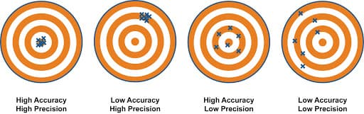
The main metrics I used were precision and recall. Precision is how often a kick predicted to be a goal actually results in a goal. Recall is the fraction of all actual goals that our model correctly predicted to result in goals.
While iterating over features, I had to compare the model with all features and different combinations of the features. Here is one of the final comparisons I did.
| Model | Parameters | Accuracy | Precision | Recall | AUC ROC | Features |
|---|---|---|---|---|---|---|
| Random Forest | max_depth=12 | 0.97 | 0.747 | 0.163 | 0.581 | goal_distance,goal_angle, defender_dist, closest_defender, defenders_within_box, in_box, in_shot, ball_speed |
| Random Forest | max_depth=12 | 0.966 | 0.484 | 0.066 | 0.532 | goal_distance, goal_angle |
| Random Forest | max_depth=12 | 0.97 | 0.66 | 0.231 | 0.613 | goal_distance, goal_angle, defender_dist, in_shot, ball_speed |
| Random Forest | max_depth=12 | 0.97 | 0.636 | 0.229 | 0.612 | goal_distance, goal_angle, defender_dist, closest_defender, ball_speed |
| Random Forest | max_depth=12 | 0.969 | 0.612 | 0.22 | 0.607 | goal_distance, goal_angle, ball_speed |
The final features I chose were:
- Goal Distance (numerical): the distance from the ball to the goal.
- Goal Angle (numerical): the angle in radians between the line of the shot and the goal line, 0 for parallel to the goal line, pi/2 for perpendicular to the goal line.
- Defender within a distance (numerical): The number of defenders within a predefined distance from the ball.
- Closest Defender (numerical): The distance to the closest defender.
- Players within a box (numerical): The number of players in a rectangle coming out from the goal to the ball.
- Player in box (boolean): Whether there are any players within the rectangle created by defenders_within_box.
- Player in shot (boolean): Whether there are any players within the rectangle created by defenders_within_shot.
- Ball speed (numerical): Speed of the ball within a 1 second interval using distance over time.
The only feature I did not include was players within the shot.
Did my features improve the model?
The way to test the question above is to perform an ablation test where I remove all the features and run the same model on both features.
In the image below, we have a comparison of the model with my features vs the original model.
| Model | Parameters | Features | Accuracy | Precision | Recall | AUC ROC |
|---|---|---|---|---|---|---|
| Random Forest | max_depth=12 | goal_distance,goal_angle, defender_dist, closest_defender, defenders_within_box, in_box, in_shot, ball_speed | 0.97 | 0.747 | 0.163 | 0.581 |
| Random Forest | max_depth=12 | goal_distance,goal_angle | 0.966 | 0.484 | 0.066 | 0.532 |
The data shows that any model on the original data without any features had no chance at predicting XG precisely.
Once I thought the features created a model that was good at predicting XG, I deployed that model to the website, located here.
Why my model is a good model
As we can see above, our model is good based on metrics, but why does the random forest classifier perform the best?
Let’s compare Random Forest to Gradient Boost, since these models performed the best and worst respectively at the task of predicting XG. These two models were both ensemble methods
Ensemble learning is an approach to machine learning where multiple weaker models are used to create a better final model.
What is the difference between these two ensemble methods?
Random forest uses bagging, which focuses on learning from the weaker models independently and trying to combine them in a deterministic averaging process.
Gradient Boost uses boosting, which focuses on learning from the weaker models and trying to create the final best model sequentially.
Roughly speaking, bagging focuses on averaging out the weaker models to create the final model, while boosting focuses on learning upon other features sequentially.
If you want to learn more, check out this article
Discussion
We have to contextualize the problem and the results. We know that our model is good and some reasons as to why the model performed better than the other models, but why did those specific features create a model that was good at predicting XG?
I believe these features worked well because there are certain features are necessary conditions for a goal to happen. You have a higher chance of scoring if you are closer to the goal, you can’t score if players are between you and the goal, if the ball is moving fast you have a higher chance of scoring since the ball will catch the opponent off guard and unable to react.
Above was my hypothesis as to why certain features made our model better than others. The most important feature of my model was the speed of the ball, boosting the model's precision by a significant amount. This can be seen below by ball_speed's SHAP value.
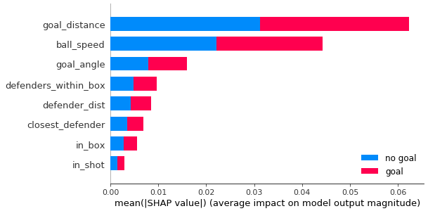
Feature importance help us understand how much each feature contributes to the model’s prediction. We often want interpretable models as we want to be to explain these models to people from a non-technical background. SHAP (SHapley Additive exPlanations) is a game theoretic approach to explain the output of any machine learning model. SHAP is similar to feature importance which shows us how the features impact the model. SHAP uniquely allow us to view how features impact individual predictions and then averages these impacts on the model’s predictions.
If you want to learn more, check out this article.
Feedback
My feedback came from high school students who are taking a course on sports analytics and got to view the model’s XG predictions for games of HaxBall that they played.
These students were able to notice some errors in our model. We had measurement errors due to kicks from the match they played not recorded by our headless API.
I received feedback about the scores of XG being too low. A kick is never certain to go in, even at goal lines. To the students/players, they believed that a value of 0.6 is too low for a kick right on goal line. I could have done some post modeling adjustments to improve the score distributions.
Challenges
Some of the challenges I ran into include typical machine learning or software engineering issues where you don’t know the value a certain feature will add so will it be better to spend more time on a feature you think will provide value or iterate quickly over a smaller feature that you think will bring value.
Most of the project challenges came down to this project being crammed into 2 weeks during the winter holiday season.
I had a couple features I wanted to work on such as whether a Fast Break was occurring, a boolean value to tell if a speed of the ball was greater than 100 m/s and ended up in the opponent's half, but my heuristic was poor or the feature was too similar to the other features, thus not really having an impact on the model’s performance.
There were other features I wanted to implement such as time length of a possession, and splitting the field into sectors.
I probably could have tuned the parameters for the random forest classifier to optimize the results of the model as well.
Things I Enjoyed about this project
Disclaimer: Data science is not my main area of expertise. I enjoy back-end web development and info/system/network security.
I enjoyed being able to work in a one-on-one environment, receive feedback and advice on the model and overall software engineering.
Most of the things I enjoyed were the same things that made this project unique, such as being able to see my results on a website.
I was glad to see that my model was good at predicting XG compared to the original model and compared to any metric.
When we performed the [ablation test above](#Did my features improve the model?). We saw that the model without our features did not perform nearly as well at the task of predicting XG.
I learned a lot about making interpretable data science results. Also, areas in my software engineering skill set that I can improve on!
Links and References
If you want to see the website where my model is deployed, you can go here!
If you want to see some examples of my model, here is an example.
If you want to see some of the work I did you can check out the HaxML repository on Github.
Some of the tools I used that you are probably familiar with:
Thank you to Vinesh Kannan for giving me the chance to work on this project.